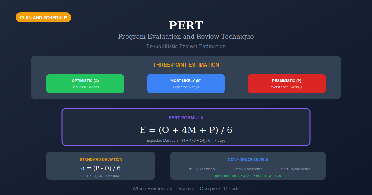
PERT: Probabilistic Project Estimation
PERT (Program Evaluation and Review Technique) uses three-point estimates—Optimistic (O), Most Likely (M), and Pessimistic (P)—to calculate expected duration and standard deviation, enabling probability-based scheduling.
Before you start
Is PERT your framework?
PERT suits work where durations are genuinely uncertain and the sequence is fixed — research, engineering development, construction, anything done rarely enough that nobody can quote a reliable duration from experience.
Its distinctive contribution is treating each duration as a range rather than a number. Everything else it does, the critical path method does too, and does deterministically.
| If your real problem is… | You probably want |
|---|---|
| Durations are well known and we need the critical path | Critical Path Method — deterministic, single estimate per activity Compare PERT and CPM |
| We need to show a schedule to people, not compute one | Gantt Chart — presentation, not estimation Not sure which? Compare |
| We do not yet know what the activities are | Work Breakdown Structure — PERT needs a complete activity list as input |
| Scope changes constantly and sequence is not fixed | Kanban or Sprint Planning — network models assume a stable plan Not sure which? Compare |
| One step is clearly the constraint | Theory of Constraints |
| Sequence is fixed and durations are honestly uncertain | PERT — you are in the right place |
PERT or CPM: the actual difference
PERT is probabilistic; CPM is deterministic. PERT takes three time estimates per activity and produces an expected duration with a variance. CPM takes one estimate per activity and produces a single answer. In practice most modern scheduling tools blend them — a CPM network with PERT-weighted estimates — which is why the two names are so often run together as “PERT/CPM”.
What Is It?
PERT acknowledges that task duration estimates are inherently uncertain. Instead of a single-point estimate, you provide three: the best case (Optimistic), the most likely outcome, and the worst case (Pessimistic). The formula E = (O + 4M + P) / 6 calculates the expected duration.
The technique also calculates standard deviation σ = (P - O) / 6, enabling you to express completion dates with confidence levels (e.g., "95% confident we'll finish by date X").
PERT connects to CPM for network analysis, WBS for task definition, and Gantt Charts for visualization.

Quick Reference
The core calculation
The PERT formula
Three estimates per activity: O optimistic, M most likely, P pessimistic. From those, three numbers.
| Quantity | Formula | What it gives you | What it assumes |
|---|---|---|---|
| Expected time (tE) | (O + 4M + P) ÷ 6 | A single duration weighted four-to-one toward the most likely case | That activity duration follows a beta distribution. The weighting was chosen for tractability, not derived — see the evidence below. |
| Standard deviation (σ) | (P − O) ÷ 6 | How uncertain that activity is | That the full range spans roughly six standard deviations, so σ is read straight off the range rather than derived from a variance. |
| Variance (σ2) | ((P − O) ÷ 6)2 | The quantity you add along a path — standard deviations do not add, variances do | That activity durations are statistically independent. |
Why is there no square root in the activity formula? Because PERT runs the usual definition backwards. Normally you compute a variance from data and take its square root to get the standard deviation. Here there is no data — so σ is estimated directly from the range, on the assumption that optimistic-to-pessimistic spans about six standard deviations, roughly ±3σ either side of the mean. That gives σ = (P − O) ÷ 6 in one step, and variance is then obtained by squaring it — the reverse of the familiar order.
The square root appears exactly once, at the end. For a whole path: sum the expected times, sum the variances, then take the square root of that total to get the path standard deviation. Project duration is then treated as normally distributed, which lets you state a completion date with a confidence level rather than a single date.
The trap in that last step
The probability figure applies to one path, not to the project. Where several paths converge, the project finishes when the slowest of them does, and the expected value of a maximum is larger than the maximum of the expected values. PERT computed on the single longest expected path therefore runs systematically optimistic. This is known as merge bias, it was documented in 1964, and it is the single most important thing to know about the technique.
Core Features
- Three-Point Estimates: Optimistic, Most Likely, Pessimistic for each task
- Weighted Average: Formula weights most likely estimate 4x
- Standard Deviation: Measures estimate uncertainty per task
- Confidence Intervals: Probability of meeting specific dates
- Network Integration: Works with critical path analysis
- Risk Communication: Expresses schedule risk quantitatively
Worked example
A PERT calculation, start to finish
An illustrative composite: five activities on a single path, durations in working days. This is the arithmetic in full, including the step most examples skip.
| Activity | O | M | P | tE = (O+4M+P)/6 | σ = (P−O)/6 | Variance |
|---|---|---|---|---|---|---|
| Requirements | 5 | 8 | 17 | (5+32+17)/6 = 9.0 | 2.00 | 4.00 |
| Design | 10 | 12 | 20 | (10+48+20)/6 = 13.0 | 1.67 | 2.78 |
| Build | 15 | 20 | 49 | (15+80+49)/6 = 24.0 | 5.67 | 32.11 |
| Integrate | 4 | 6 | 14 | (4+24+14)/6 = 7.0 | 1.67 | 2.78 |
| Test | 6 | 9 | 18 | (6+36+18)/6 = 10.0 | 2.00 | 4.00 |
| Path total | — | — | — | 63.0 days | √45.67 = 6.76 | 45.67 |
Expected duration is 63 days with a standard deviation of 6.76 days. Because durations are treated as normally distributed at path level, that converts directly into confidence:
- 50% confidence: 63 days — the expected value, and a coin flip
- 84% confidence: 63 + 6.76 ≈ 70 days (one standard deviation)
- 95% confidence: 63 + (1.645 × 6.76) ≈ 74 days
What the numbers actually tell you
Two things worth noticing. First, quoting 63 days means promising a date you will miss half the time — the expected value is a median-ish figure, not a commitment. If you need to be reliably right, quote 74.
Second, look at the variance column. Build contributes 32.11 of the 45.67 total — about 70% of all the uncertainty in the project sits in one activity, entirely because its pessimistic case is 49 days against a most likely of 20. That is where estimation effort and risk mitigation belong. Averaging attention across all five activities would be a mistake the arithmetic has already warned you about.
When to Use
- Research and development projects
- New product development with unknowns
- Projects with significant uncertainty
- When stakeholders need confidence intervals
- Government and defense projects
- First-time or unique project types
- Risk-sensitive environments
When NOT to Use
- Routine, well-understood projects
- When historical data provides reliable estimates
- Simple projects with few tasks
- When the added complexity isn't justified
- Teams unfamiliar with statistical concepts
In practice
How PERT estimates go wrong
The arithmetic is reliable. The inputs and the interpretation are where projects come unstuck.
| What you see | What it usually means | What to do |
|---|---|---|
| P is only slightly larger than M | The pessimistic case is a mild inconvenience, not a genuine worst case | Ask what happens if the key person leaves, the vendor slips, or the approach fails and you restart. Real distributions are strongly right-skewed; a symmetric three-point estimate is a warning sign. |
| The project is quoted at the expected duration | A 50%-confidence figure is being treated as a commitment | Quote a confidence level with the date, or quote expected time plus one to two standard deviations. Never present tE alone to a stakeholder who will treat it as a promise. |
| Standard deviations were added along the path | A common arithmetic error | Variances add; standard deviations do not. Sum the variances, then take the square root once at the end. |
| Probability quoted for the project, computed on one path | Merge bias — the near-critical paths were ignored | Any path within about one standard deviation of the critical path can become critical. With several such paths the true completion probability is materially lower than the figure PERT reports. Simulate if the stakes justify it. |
| Estimates came from whoever was in the room | The three points are guesses wearing a formula | PERT propagates the estimates faithfully; it cannot improve them. Get them from people who have done the work, and separately from someone with no stake in the answer. |
| Built once and never revised | Treated as a plan rather than a model | Re-estimate remaining activities as uncertainty resolves. The variance on a finished activity is zero, and the whole distribution should tighten as the project proceeds. |
Sourced
What the evidence says
The founding paper is Malcolm, Roseboom, Clark and Fazar, 1959.
PERT was developed in 1958 for the US Navy’s Special Projects Office on the Polaris fleet ballistic missile program, and published the following year in Operations Research. If you need a citable primary source for the technique or the three-estimate approach, this is it — not a textbook and not a wiki.
Malcolm, D. G., Roseboom, J. H., Clark, C. E. & Fazar, W., “Application of a Technique for Research and Development Program Evaluation”, Operations Research 7(5), Oct 1959, pp. 646–669.
The four-to-one weighting was chosen for convenience, not derived.
The beta distribution was adopted because its parameters can be recovered algebraically from the two extremes and the mode — Clark justified the choice on grounds of tractability in 1962. The question of where the weights in (O + 4M + P)/6 actually come from was still being asked in the literature decades later: Sasieni raised it in Management Science in 1986, prompting replies from Littlefield and Randolph and from Gallagher in 1987. The formula is a workable approximation with a convenient shape, not a result derived from the behavior of real projects.
Sasieni, M. W., “A Note on Pert Times”, Management Science 32(12), 1986; replies in Management Science 33(10), 1987.
PERT is systematically optimistic, and this was established in 1964.
MacCrimmon and Ryavec analyzed the model’s assumptions and identified three separate sources of error at activity level: that real durations are not beta distributed, that the approximation formulas introduce error of their own, and that the expert estimates feeding them are imprecise. More seriously, at network level they showed that computing project duration from the path with the largest sum of expected times produces overly optimistic results, because where paths converge the project waits for the slowest, and the expected value of a maximum exceeds the maximum of expected values. This is merge bias. It means a PERT figure is a floor rather than a forecast.
MacCrimmon, K. R. & Ryavec, C. A., “An Analytical Study of the PERT Assumptions”, Operations Research 12(1), 1964, pp. 16–37. RAND memorandum
Its most famous success story is largely a myth.
PERT is routinely credited with pulling the Polaris program years ahead of schedule. Harvey Sapolsky’s study of that program found something different: PERT was, in his account, as much a device to protect the program from outside interference as an effective management tool — a technique whose visible sophistication kept reviewers and political overseers at a distance. Not even a majority of Polaris tasks were actually controlled through it. The program succeeded; the evidence that PERT is why is thin.
Sapolsky, H. M., The Polaris System Development: Bureaucratic and Programmatic Success in Government, Harvard University Press, 1972.
What that means for using it.
None of this makes PERT useless, and it is worth being clear about that. Forcing three estimates surfaces uncertainty that a single number hides, and the variance column tells you where the risk actually concentrates — both genuinely valuable, and neither dependent on the distribution being exactly right. What the evidence does say is that the output is a floor, not a forecast: quote it with a confidence level, watch the near-critical paths, and treat the probability figure as directional. Used that way it is a good instrument. Used as a precise prediction, it will be wrong in a predictable direction.
Key Strengths
- Uncertainty Handling: Explicitly models estimate uncertainty
- Risk Communication: Expresses schedules with confidence levels
- Better Estimates: Forces consideration of best/worst cases
- Statistical Foundation: Mathematically sound approach
- Stakeholder Buy-in: Transparent about uncertainty
Key Weaknesses
- More complex than single-point estimation
- Requires three estimates per task (time-consuming)
- Assumes beta distribution may not always fit reality
- Can give false precision if estimates are poor
- Historical data often limited for calibration
How It Works
| 1 Primary Input | Three estimates per task: Optimistic, Most Likely, Pessimistic |
|---|---|
| 2 Data You Need | Task list, expert judgment, historical data where available |
| 3 Primary Output | Expected duration, standard deviation, confidence intervals, risk-adjusted schedule |
Comparison with Related Frameworks
PERT vs Critical Path Method
CPM uses deterministic single-point estimates, while PERT uses probabilistic three-point estimates. Use CPM for well-understood construction work; PERT for R&D and uncertain projects.
PERT vs Work Breakdown Structure
WBS defines what tasks exist; PERT estimates how long they'll take with uncertainty. WBS is the input; PERT is the analysis. Use both together for comprehensive project planning.
Sequencing
What to run before and after
PERT is a calculation applied to a plan. It needs the plan built first, and it produces numbers that something else has to act on.
Before
Decompose the work and fix the sequence
PERT takes a complete activity list with dependencies as input. Miss an activity and no amount of statistical sophistication downstream will find it.
During
Find the critical path, then quantify it
CPM identifies which path drives the schedule; PERT tells you how confident you can be about it. This is why the two are usually taught and used together.
After
Manage the variance you found
The variance column names your highest-risk activities before anything has gone wrong. That is a risk register with the priorities already computed.
Common questions
PERT: quick answers
What is the PERT formula?
Expected time tE = (O + 4M + P) ÷ 6, where O is the optimistic estimate, M the most likely and P the pessimistic. Standard deviation σ = (P − O) ÷ 6, and variance = ((P − O) ÷ 6)². Along a path, sum the expected times and sum the variances, then take the square root of the total variance — variances add, standard deviations do not.
Why is there no square root in the PERT standard deviation formula?
Because σ is not being derived from a variance here. With no historical data to compute one, PERT estimates the standard deviation directly from the range, assuming optimistic-to-pessimistic covers about six standard deviations — giving σ = (P − O) ÷ 6 in a single step. Variance is then found by squaring that, which reverses the usual order. The square root is needed only once, at the end: sum the variances along a path, then take the square root of that total to get the path standard deviation.
Is PERT probabilistic or deterministic?
Probabilistic. PERT takes three time estimates per activity and produces an expected duration with a variance, letting you state completion dates with a confidence level. The Critical Path Method is deterministic: one estimate per activity, one answer. That distinction is the main difference between the two techniques, which is why they are often taught together as PERT/CPM.
What is the difference between PERT and CPM?
PERT is probabilistic and uses three time estimates per activity; CPM is deterministic and uses one. PERT was developed in 1958 for the US Navy’s Polaris program where durations were genuinely unknown; CPM emerged around the same time for industrial projects where durations were well understood from experience. Most modern scheduling tools blend the two: a CPM network with PERT-weighted estimates.
Where does the (O + 4M + P) / 6 formula come from?
It approximates the mean of a beta distribution. The beta was chosen largely because its parameters can be recovered algebraically from the two extremes and the mode — a matter of tractability rather than evidence about real project durations. The origin of the specific weighting was still being debated in Management Science in 1986 and 1987. Treat it as a workable approximation, not a derived result.
Does PERT underestimate project duration?
Yes, systematically. MacCrimmon and Ryavec showed in 1964 that calculating project duration from the path with the largest sum of expected times gives overly optimistic results. Where parallel paths converge the project waits for the slowest one, and the expected value of a maximum exceeds the maximum of the expected values — known as merge bias. Treat a PERT figure as a floor rather than a forecast, and quote it with a confidence level.
Did PERT really save two years on the Polaris program?
Probably not. That claim is repeated constantly and the evidence for it is thin. Harvey Sapolsky’s study of the program concluded PERT was as much a device to protect it from external interference as an effective management tool, and that not even a majority of Polaris tasks were actually controlled through PERT. The program succeeded; attributing that success to PERT is a separate claim that has not been established.
Deep Resources
Frameworks related to PERT (Program Evaluation and Review Technique)
- Critical Path Method (CPM)Network analysis identifying longest dependent activity sequence to determine minimum project…
- Work Breakdown Structure (WBS)Framework for decomposing complex projects into hierarchical, manageable components for…