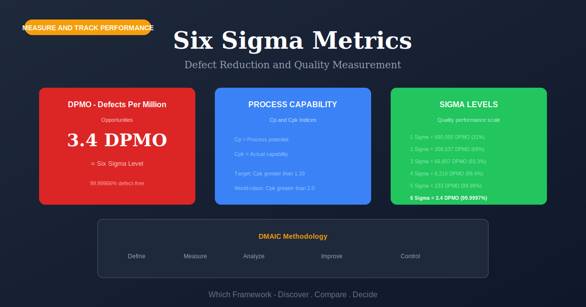
Six Sigma Metrics: DPMO, Sigma Levels, and a Defect Rate You Can Defend
Six Sigma Metrics are measures that quantify process quality against specification limits, comprising defects per unit, defects per million opportunities, yield, sigma level and the capability indices Cp and Cpk.
Before you start
Is this your framework?
This page is about expressing quality as a number and knowing what that number rests on. Sigma levels, defects per million, yield, and the assumptions buried in each.
It is measurement, not improvement. Knowing you are at 3.8 sigma tells you where you stand and nothing about how to move. The table below routes to the methods that do that.
| If your real problem is… | You probably want |
|---|---|
| We know the defect rate and need to reduce it | Lean Six Sigma — the DMAIC cycle, which uses these metrics in its Measure phase Compare Six Sigma Metrics and Lean Six Sigma |
| We need to choose which measures the business reports on generally | Key Performance Indicators — selecting and owning measures, of which defect rates are one kind Compare Six Sigma Metrics and KPIs |
| We want to know how we compare with others, not just our own trend | Benchmarking — external comparison, where the like-for-like problem is the hard part |
| The process is slow rather than defective | Value Stream Mapping — waiting and flow, which no defect metric will surface |
| We need these numbers on a screen people actually look at | Dashboarding and Visualization — presentation and cadence rather than definition |
| Small continuous improvements by the people doing the work | Kaizen — short cycles that need far less measurement apparatus |
| We need to state our quality as a defensible number, and know what it assumes | Six Sigma Metrics — you are in the right place |
What Is It?
The idea is to express quality as one comparable number, so a wiring harness and an invoice can be discussed on the same scale. Count what went wrong, divide by how many chances there were for something to go wrong, and scale it to a million. That gives defects per million opportunities, and from it a sigma level.
The sigma level is a count of standard deviations between the process mean and the nearest specification limit. More sigma means more room before the process produces something out of tolerance. Six sigma means six standard deviations of room, and the method took its name from that target.
Six standard deviations of room, on a stable centered process, gives about two defects per billion. Not 3.4 per million. Both figures are in circulation, they differ by a factor of about seventeen hundred, and most published tables print one without saying which.
The difference is an assumption. Motorola built in an allowance for processes drifting over time, standardized at 1.5 sigma, on the grounds that short-run data flatters a process that will wander over months. Apply that allowance and six sigma reports as 3.4 defects per million. The number everyone quotes is a long-term figure with a drift assumption inside it.
None of this makes the metrics unusable. It makes them conventions rather than facts, and conventions have to be stated. A defect rate is only comparable to another defect rate if both used the same definition of a defect, the same count of opportunities, and the same assumption about drift — and in practice, published rates rarely say which.
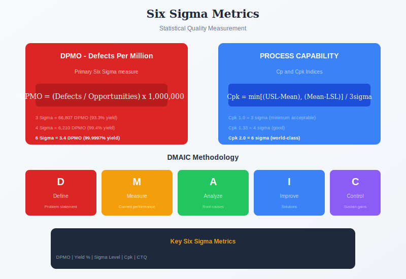
Quick Reference
The numbers
The table, and the shift inside it
Both columns below describe the same processes. They differ only in whether the 1.5 sigma drift allowance has been applied. The left column is what you get from a normal distribution; the right is what the industry quotes.
| Sigma level | Short-term DPMO no shift applied | Long-term DPMO 1.5 sigma shift, the quoted figure | Long-term yield |
|---|---|---|---|
| 1 | 317,311 | 691,462 | 30.85% |
| 2 | 45,500 | 308,538 | 69.15% |
| 3 | 2,700 | 66,807 | 93.32% |
| 4 | 63 | 6,210 | 99.38% |
| 5 | 0.57 | 233 | 99.977% |
| 6 | 0.002 | 3.4 | 99.99966% |
What the 3.4 actually is
The long-term column is computed by taking the one-sided tail of the normal distribution at the sigma level minus 1.5. So the 3.4 figure at six sigma is really the tail at 4.5 sigma. The number that names the entire methodology corresponds to four and a half standard deviations, not six. Anyone who tries to reproduce 3.4 from a statistics table and fails has done the arithmetic correctly.
The convention exists for a defensible reason. Short-term data collected over a project captures common-cause variation only, and Motorola's observation was that real processes drift by something between 1.4 and 1.6 sigma over longer periods. Whether that generalizes beyond the processes it was observed on has been argued about ever since. Treat 1.5 as an industry default you may need to defend, not as a property of nature.
Choosing
Which metric answers which question
Several measures get used interchangeably and answer different questions. The distinction that matters most is between measures that account for complexity and measures that do not.
| Measure | What it answers | What it hides |
|---|---|---|
| DPU defects per unit | How many faults on an average unit. Simple and needs no judgment calls. | Complexity. A hundred-component assembly and a two-field form are not comparable on this scale. |
| DPMO per million opportunities | A rate normalized for complexity, so different processes can be compared. | The definition of an opportunity, which is a judgment call. Count more opportunities per unit and the rate improves without anything changing. |
| Yield first pass | The proportion that got through one step without rework. | Everything before and after that step. Flattering for any single stage in a long process. |
| Rolled throughput yield | The proportion getting through every step untouched, found by multiplying the step yields. | Nothing much, which is why it is the uncomfortable one. Ten steps at 99% each gives about 90% overall. |
| Sigma level | Distance to the nearest specification limit, in standard deviations. | Whether the shift was applied, and whether the data was short-term or long-term. |
| Cp and Cpk | Capability against the specification. Cpk also accounts for the process being off-center. | Less than the others, which is why engineers prefer them. Reported short-term, without a shift. |
The opportunity count is where the number gets soft
DPMO's normalization is genuinely useful and genuinely manipulable. If a unit has twelve solder joints, is that twelve opportunities or one? Both answers are arguable, and they differ by a factor of twelve in the reported rate. Nothing about the process changes; only the denominator does.
Two habits keep this honest. Fix the opportunity definition in writing before any baseline is taken, and treat any later change to it as resetting the baseline rather than improving the number. And when comparing your rate against anyone else's, ask how they counted opportunities before concluding anything. Most published comparisons cannot answer that.
Core Features
- A written definition of a defect: the boundary between acceptable and not
- A fixed opportunity count: agreed before the baseline, changed only by resetting it
- A stated time basis: short-term or long-term, since the two differ enormously
- A stated shift assumption: whether 1.5 sigma has been applied
- A validated measurement system: evidence that two observers agree
- Rolled throughput yield for multi-step work: the figure single-step yields conceal
Worked example
4.1 sigma that turned out to be 2.6
An illustrative composite. An electronics assembler in Penang, Malaysia, building control boards for industrial customers. The quality report showed 4.1 sigma and had done for two years. A customer audit asked how the figure was derived, and the answer took three weeks to assemble.
| Question asked | What it turned out to be |
|---|---|
| How many opportunities per board? | Every solder joint and every component placement had been counted: 1,180 per board. A defensible choice that made the DPMO rate look excellent. Counting only functional test points, as their customer did, gave 46 opportunities and a very different number. |
| Short-term or long-term? | The 4.1 sigma had been calculated from a normal table with no shift applied, then reported alongside industry figures that all included one. Like for like, the process was closer to 2.6 sigma. |
| What was the yield across all steps? | Nine steps were each reported above 98%. Rolled throughput yield was 84.4%, a number nobody had ever computed because no single report spanned the whole line. |
| Would two inspectors agree? | On cosmetic solder criteria, agreement was 78%. On functional failures it was near total. The cosmetic category was roughly a third of all recorded defects. |
| What changed | Opportunity count fixed at functional test points and written into the quality plan. Reporting switched to long-term with the shift stated on the page. Rolled throughput yield added as the headline. Cosmetic criteria rewritten with photographs. |
Nothing on the line changed, and every number did
The reported sigma level fell from 4.1 to 2.6 and the headline yield fell from "above 98%" to 84.4%. No process was altered during the audit. The old figures were not fabricated; each was computed correctly under an assumption that had never been written down, and the assumptions had drifted apart from the ones their customer used.
The most useful output was not a better number but a shorter list of them. One defect definition, one opportunity count, one time basis, one headline figure covering the whole line. A quality metric that cannot survive being asked how it was calculated is not a measurement, it is a claim — and it had passed two years of management review without anyone asking.
When to Use
- Repetitive work with enough volume for a rate to be meaningful
- A defect can be defined unambiguously and observers would agree
- You need to compare quality across processes of different complexity
- Setting a contractual or customer quality commitment
- Establishing a baseline before a DMAIC project
- A multi-step process where per-step yields look better than reality
When NOT to Use
- Low volume or bespoke work, where a rate has nothing to average over
- Quality that is a matter of judgment rather than conformance
- Where the opportunity count cannot be agreed and would be arbitrary
- As an individual or team performance measure, where it will be gamed
- Creative or exploratory work, where variation carries the value
- Comparing against outside figures whose definitions you cannot see
In practice
How the numbers go wrong
Almost all of these are the same failure: an assumption that was reasonable when made, never written down, and later compared against figures built on a different one.
| Failure mode | What it looks like | What to do instead |
|---|---|---|
| Opportunity inflation | The rate improves after somebody recounts what a defect opportunity is | Fix the count in writing. Any change resets the baseline and is annotated, not celebrated. |
| Mixing short-term and long-term | An internal figure with no shift compared against published figures that all include one | State the basis on every report. A number without it cannot be compared with anything. |
| Single-step yield as the headline | Every stage above 98% while the line as a whole is nearer 85% | Report rolled throughput yield. It is the number the customer experiences. |
| Unvalidated inspection | A defect rate built on criteria two inspectors read differently | Check agreement first. Rewrite subjective criteria with examples before trusting any rate. |
| Chasing six sigma everywhere | Enormous effort pushing a process well past what the customer would pay for | Set the target from the economics. Four sigma is a defensible answer in most service work. |
| Metrics tied to pay | Reported defects fall while customer complaints do not | Keep defect rates out of bonus formulas. They are unusually easy to influence at the point of recording. |
Sourced
Evidence, and how to cite it
A true six sigma process is about 0.002 defects per million, not 3.4.
Six standard deviations of room on a stable, centered process gives roughly two defects per billion opportunities. The quoted 3.4 per million is the one-sided normal tail at 4.5 sigma, which is what six sigma becomes once Motorola's 1.5 sigma drift allowance is subtracted. The figure that names the methodology therefore describes four and a half sigma of capability, not six. This is not obscure, but it is left out of most published tables, which is why the arithmetic appears not to work.
Standard normal distribution; the conventional long-term sigma table as used across Six Sigma practice.
The 1.5 sigma shift is a convention derived from observation, not a statistical result.
Motorola's argument was that short-term data captures common-cause variation only, while over longer periods special causes move the process mean. Their observed drift was around 1.4 to 1.6 sigma, and 1.5 was adopted as the standard allowance. Whether a figure observed in particular manufacturing processes should be applied universally has been contested in the quality literature for decades. It is best treated as an industry default you should be ready to defend, and one you should always state.
Motorola Six Sigma reporting convention; ongoing discussion in the statistical quality control literature.
The program has a specific origin and date.
Bill Smith, a reliability engineer at Motorola, argued in a mid-1980s memo that product field life was tied to rework during manufacturing. Chief executive Bob Galvin backed the idea against most of his senior team. Motorola launched the program formally on 15 January 1987 with a target of fewer than 3.4 defects per million opportunities, and won the first Malcolm Baldrige National Quality Award in 1988. The 3.4 target was therefore set with the shift already assumed.
Contemporaneous accounts of the Motorola Six Sigma program; Smith, W.B. (1929–1993), Motorola.
DPMO can be improved without improving anything.
The denominator is a judgment. A circuit board can reasonably be described as having a thousand defect opportunities or fifty, depending on whether you count every joint or only the functional tests. The reported rate changes by a factor of twenty and the process does not change at all. This is the same structural problem as any measure used as a target, and it is why defect rates should be kept out of incentive schemes and why cross-company comparisons need the opportunity definition before they mean anything.
Standard DPMO definition; see also the literature on measures that become targets.
How to cite it.
Harvard: Montgomery, D.C. (2009) Introduction to Statistical Quality Control. 6th edn. Hoboken: Wiley.
APA: Montgomery, D. C. (2009). Introduction to statistical quality control (6th ed.). Wiley.
For the sigma table and the target, cite the Motorola program under Bill Smith, launched January 1987. Always state whether your figures are short-term or long-term, since the two differ by a factor of thousands at the top of the table.
Key Strengths
- Comparable across complexity: a harness and an invoice on one scale
- Forces a written definition: of what counts as a defect, which is valuable on its own
- Rolled throughput yield is honest: it exposes what per-step figures conceal
- Well understood: customers and auditors know what a sigma level means
- Cheap once defined: the cost is in agreeing the definitions, not in the arithmetic
Key Weaknesses
- The opportunity count is a judgment: and moves the answer by an order of magnitude
- The headline figure hides an assumption: 3.4 is a shifted, long-term number
- Comparisons are usually invalid: published rates rarely state their basis
- Needs volume: a rate over a handful of units means very little
- Easy to influence at the point of recording: which makes it a poor incentive measure
Sequencing
What to run before and after
These metrics sit between defining what quality means and doing something about it. Neither neighbour is optional.
Before
Agree what a defect is, and check people apply it the same way
Every number here rests on a defect definition and an opportunity count. If two inspectors disagree, the rate measures the disagreement rather than the process.
During
Use the baseline to drive an improvement cycle
A sigma level tells you where you stand and nothing about how to move. The Measure phase of a DMAIC project is exactly where these numbers earn their cost.
After
Report it where it will be read, and compare carefully
State the basis on every report. Before comparing against anyone else's figure, find out how they defined an opportunity and whether they applied the shift.
Common questions
Six Sigma metrics: quick answers
What is DPMO?
Defects per million opportunities. Count the defects found, divide by the number of units multiplied by the opportunities for a defect in each unit, then multiply by a million. It scales across processes of different sizes, which is its point, and it depends entirely on how you define an opportunity, which is its weakness.
How many defects per million is six sigma?
3.4, by the usual convention. That figure already includes an assumed 1.5 sigma long-term drift in the process mean. Without that assumption a six sigma process is about 0.002 defects per million, or two per billion. The 3.4 figure actually corresponds to 4.5 sigma, which is why the arithmetic never works when people try to reproduce it from a normal distribution table.
What is the 1.5 sigma shift?
An allowance Motorola built in for processes drifting over time. Short-term data captures only common-cause variation; over months, special causes shift the mean. Motorola put the typical drift at roughly 1.4 to 1.6 sigma and standardized on 1.5. It is a reporting convention derived from observation rather than a statistical law, and it has been disputed in the literature ever since.
What is the defect rate at 3 sigma?
66,807 defects per million by the long-term convention, or about 93.3% yield. Without the 1.5 sigma shift the same level is roughly 2,700 per million. The gap between those two numbers is why quoted defect rates for the same process can differ by more than an order of magnitude depending on which table the author copied.
What is the difference between DPU, DPMO and yield?
DPU is defects per unit, which ignores how complex a unit is. DPMO divides by opportunities, so it can compare a wiring harness with an invoice. Yield is the proportion passing. Rolled throughput yield multiplies the yields of every step, which is the honest figure for a multi-step process and is always worse than any single step suggests.
What is the difference between sigma level and Cpk?
Both describe how much room a process has inside its specification limits. Sigma level is the count of standard deviations to the nearest limit and is usually quoted with the shift applied. Cpk measures the same distance but accounts for the process being off-center, and is reported short-term without a shift. As a rough guide, a Cpk of 2.0 corresponds to six sigma.
Is six sigma a realistic target?
For high-volume repetitive manufacturing it is achievable and sometimes already exceeded. For most service and transactional processes it is not, and pursuing it is rarely worth the cost. Four sigma, at about 6,210 defects per million, is a common and defensible target. The sensible question is what defect rate the customer and the economics justify, not what the name of the method implies.
How do you cite six sigma metrics?
For the sigma table and the shift, cite Motorola's Six Sigma program under Bill Smith, launched January 1987. For process capability definitions, cite a standard text such as Montgomery's Introduction to Statistical Quality Control. State explicitly whether your figures are short-term or long-term, because the two differ by a factor of thousands at the top of the table.
Deep Resources
Frameworks related to Six Sigma Metrics
- Lean Six SigmaThe DMAIC cycle these metrics feed, and the Lean half that defect rates never surface…
- Key Performance IndicatorsChoosing which measures to report at all, of which defect rates are one kind…
- BenchmarkingComparing your rate against others, where differing definitions are the hard part…